Watch: TESCAN Dynamic microCT

Learn the basics of microCT and dynamic image capture for dynamic process views in the laboratory.

First, a little bit of introduction to TESCAN and micro-CT. TESCAN is, modern history is about 30 years, but it goes back into the '50s with a company called Tesla, which was in the old Czechoslovakia, where they worked on a lot of the original SEM Systems and, as I mentioned, modern history is 30 years and have been focused primarily on SEM and FIBSIM. The last 10 years, there's been a lot of growth in the company with a lot of new products and techniques coming out.

From the product range in terms of SEM and FIBSIM, we have a wide portfolio. Many of you are probably familiar with thermal emission SEM, the VEGA, but we also have much higher resolution systems in the VEG SEM area. We have some special solutions for doing large samples, mineralogy, and of course our gallium and plasma FIBs, and the Plasma FIB.

From the CT side of things, the story starts 15 years ago with the University of Gent. They have a center for X-ray tomography that was established 15 years ago. For the CT portion resides in the city of Ghent and rose from that university. There were two different companies: Inside Matters, which focused a lot on software and imaging services. The other one, XRE, focused more on the development of platforms, innovative CT platforms. These two merged together in 2017, and then TESCAN acquired the company about a year later, so about two years ago, in March of 2018.

0:02:55.2: Quick snapshot of our portfolio. I'm not gonna touch too much on the specifics of the systems in this presentation. It's gonna be much more application-focused, but we have three systems: The DynaTOM, the CoreTOM, and the UniTOM XL. Down below, you'll see some specifications for these systems. The CoreTOM and the UniTOM XL are more of the traditional type of systems where the sample rotates between the source and detector. They're quite capable of imaging very large samples with fields of view up to a meter in length and 300 millimeters or larger in diameter. The DynaTOM is a much more unique system in that it is gantry-based where the source-detector actually rotates around the sample, so the sample stays stationary. And you'll see some video showing a little bit of these differences later on in the presentation.

0:03:47.1: Our big goal at TESCAN is to enable this idea of doing dynamic X-ray, 3D X-ray imaging in the lab. Something that has not been typical for really... There's been in situ and 4D that's been done in the lab, but not really a lot of dynamic CT imaging, meaning uninterrupted imaging of samples. Here on the right you see this image of this phone that's getting compressed, and it's really in an uninterrupted state, and that's really pushing more towards a real in situ capability for CT. Our systems are very capable of doing imaging of single samples, but really there's a large focus on this idea of dynamic.

0:04:28.8: Before we get too much into that, I wanna give a brief overview of the basics of micro-CT imaging. So I went into this in a lot more detail in the webinar last week, so this is just a limited region of that, but the majority of systems have the same basic components. Essentially an X-ray source, a rotation stage, and a detector. There may be different types of sources, they might be different types of detectors, but more or less all CT systems have a similar sort of architecture. Most micro-CT systems are of this flavor, where you have the rotation mount... Or the sample mounted vertically and the sample rotating. Medical CT scanners will be of a different architecture, where basically the patient or the object is laying flat and the source and detector rotate around the sample, in that direction. Our DynaTOM actually has the source and detector rotating around a vertical sample. We'll see some video of that later.

0:05:28.3: As far as the basic in terms of fundamentals, here is a little schematic of an X-ray source and a little LEGO man here that's rotating between the source and the detector. You have X-rays that penetrate and are partially absorbed by the sample. And on the detector, we're basically getting a series of 2D grayscale images that are representing essentially the transmission of X-rays through that sample. And that transmission is heavily dependent upon the attenuation of the sample, which is a function of the atomic weight and chemical composition of the material, the X-ray energy that's being used, and then the thickness of that material.

0:06:12.5: As far as resolution goes for a system, the main contributors to resolution for an overall system are the source spot, the detector pixel resolution, and then the geometric magnification, so the relationship of the sample to the source and detector, and the detector to the source. So as you move the sample closer to the source, that image is magnified and then as you move it closer to the detector it's de-magnified. It's important to note here that when you have this magnification very high, so you're very close to the source here, essentially the resolution of the system is gonna be proportional to the spot size, so the spot size of the source is an important factor in this. And the voxel size by itself is not necessarily a measurement of the resolution of a system.

0:07:04.3: So we have this series of projections that are in grayscale, they're 2D images, so everything's overlapping with one another, you can see here looking at the side view of this LEGO guy you see these overlapping features. We take those and we put them through a reconstruction algorithm that then produces a stack of 2D slices, so that's what you're seeing on the right side, essentially a stack of images that are being sliced down through from the top to bottom of this LEGO man. And you can see in these slices that you're getting a really accurate geometric reconstruction, a representation of the original object. The different grayscales in here are, again, correlated to the different attenuations of the material, which is a function of their chemistry essentially. So we see some different types of polymer in this LEGO guy.

0:07:55.2: So we have our reconstructed slice of the stack, and then we can go ahead and then create a 3D rendering from that stack, which we can manipulate in any number of directions and look at it from... Slice it through different directions, we can do analysis, voxel-based analysis looking at maybe porosity or we can do measurements of features, we can do investigation of failures like cracks and that sort of thing, so it gives us a lot of flexibility. Most importantly, it's non-destructive, so your sample is still intact. As far as dynamic CT goes, there are a couple of key components or a few key components that go into that. One is this idea of continuous rotation. So on the left here, you see a video from our DynaTOM, which is a unique system in that it has a sample mounted vertically, in this case we have a flow cell experiment going on where we have some pump pushing fluid through here and another pump providing some confining pressure. So the DynaTOM is really, really useful and this sort of configuration is very useful for more complex in-situ experiments and also for samples that are delicate in nature and are susceptible to change if you're doing some rotation to them.

0:09:09.8: On the right side, we have a video showing the inside of our UniTOM XL or CoreTOM system, and you can see here the X-ray source, this is a Deben load stage, so this is used for doing compression or tension experiments. And what's key here is that the sample is continuously rotating, and what's nice about our system here is that we have a slip ring in here we can put communication and power through to actually manage our cables a little bit better, so we don't have to worry about coiling up cables for apparatuses like this. Additionally, the stage is quite large, so we can maybe place multiple apparatuses on, we'll have an example of that a little bit later. But continuous rotation is certainly very, very key to doing these fast scans to do dynamic CT imaging.

0:09:58.6: Additionally, if you have a system that you're going to be doing a lot of in situ experimentation with and dynamic CT, you'll want to have an easy interface from the inside of the system to the outside of the system. So traditionally you have to... We've cables to do a X-ray labyrinth that's used to make sure that everything is X-ray safe, there's limited room oftentimes, and it's a bit of a hassle getting these wires through. So in our case, we have an option for an in situ interface kit, where we can actually plug in from the inside to the outside, a number of different communication and power ports, so that we can easily interface with stuff on a regular basis and multiple different types of apparatuses. So if you're doing a wide range of different types of in situ experiments, it's very nice to have this sort of interface to be able to essentially plug and play in terms of connecting the inside to the outside.

0:10:58.7: Last but not least, certainly is having special 40 tool kits to deal with this sort of data. We're collecting tens of thousands of projections in a row, basically a stream of data, and we need to be able to parse that out properly afterwards so that we can really utilize the data to its fullest extent. So there are a lot of intricacies in terms of working with this sort of data set when we're doing dynamic CT. A note on just the demand for 40 or time-dependent X-ray imaging methods, it's been interesting, we see a real uptick in the last, say, 10 years, about 10 years ago, in terms of the ratio of publications that involve temporal resolution as a major component of the experiment versus just traditional 3D X-ray imaging, and that's most likely due to the increased capabilities at Synchrotrons around the world to do faster types of scans. We probably saw something similar in the early ages of micro-CT where Synchrotron was the first facilities to do micron or sub-micron type imaging, and then that slowly went into the lab, and now we're seeing majority of dynamic CT work being done at the Synchrotrons, and now we're also pushing that into the lab. So it's an interesting transition from where we see the technology going.

0:12:21.4: But Synchrotrons themselves are these very large facilities that have limited access. I mean, these are on the order of about a half a mile circumference. I think I quoted in my last one, maybe a couple of miles, that was a little bit of an exaggeration. But in most cases, some of the largest ones can be on the order of a half mile or bigger in circumference.

0:12:43.9: There's a limited number of these around the world, but they really are very high, high intensity, billions of times brighter than things you can... Than systems in the lab. And they have unique capabilities in terms of discrete energy imaging as well, however, there's certainly limited accessibility to these... Usually you have to submit a proposal and then you can get in there maybe every six months or something for a couple of days of beam time. So you have a limited time frame to do your experiments, you can do some really awesome stuff there for sure, but it's a little bit limited.

0:13:16.9: In contrast, the lab-based systems, there are literally thousands of them around the world now, and they are, comparatively to the Synchrotron, relatively low intensity. But still you can have quite a bit of power to do fast scans. I'll show examples of scans in the order of 6 and 10 seconds today. You have 24/7 access to these systems, and they're really flexible, they're great tools, certainly as a precursor also to doing work at the Synchrotron, so making sure you iron out all of your bugs before you go to spend your two days out of a year at the Synchrotron. When we look at the physical processes that are common in material science, they span really a large range of time scales, from the very slow where you have creep centering, corrosion, etc that can be on the order of weeks or months. Even years, in some cases, to things that are very, very fast: Microseconds in terms of change.

0:14:20.7: Traditionally, the lab CT systems have done kinda time-to-minute, 4D, or time-lap studies of the slower processes, and the Synchrotron has taken care of most of the faster stuff. As we move forward, the Synchrotron is getting more and more focused really on doing the fastest type of work. In fact, there are groups out there now doing tomographies, literally 200 tomographies per second or faster, so extremely, extremely fast acquisition. And that really does allow you to get into this regime that was inaccessible previously from a 3D perspective.

0:15:00.8: What what we're trying to do is really fill in this gap here where we're looking at processes on the order of a few minutes to tens of minutes to an hour set sort of range, that has not typically been done in the lab. A couple of quick notes on the idea of temporal resolution and collecting data in a time sense. When we talk about 40, traditionally, this has meant kinda time lapse tomography where we're collecting discrete data sets over certain periods of time, at certain intervals while a process is happening.

0:15:34.6: Most of this time... Most of the time, this means this process is relatively long. The sample is changing relatively slowly, and you can collect these discrete tomography data sets. But it's really more for long kind of occurrences. As opposed to dynamic where we're more focused on faster processes, and we're really collecting data continuously throughout the whole process. So on the right side there you see an example of a sample that's continuously rotating, so we're not really thinking in terms of discrete tomography data sets at this point.

0:16:15.4: We're really thinking about just collecting a stream of projections while the sample is rotating and allowing us to collect data throughout the whole process that's happening, and this really is what is being used for looking more at the fast processes. And after the fact, after we have the data collected, we can can go in and look at what reconstruction blocks we really need. It may be every 360 degrees, it may be some portion of that, we might do some overlapping of some of these reconstruction blocks to give us some more information. So there's a lot more flexibility in terms of what you can do with the data where related to an institute experiment when you're doing this sort of data acquisition.

0:16:57.6: Alright, so that's enough background. We're gonna wanna jump now into a number of different application examples. They're gonna kinda span a wide range, and it may not apply to all of you, but hopefully you'll have some appreciation of each one. There are a couple static examples in there, but not many. It's primarily based on dynamic CT results or time lapse type of CT results. So first, let's look at a few metal examples, The first one here we saw earlier in an early slide, a video of some foam compression, here it is in a bit more detail, so here we see actually the anvils on the load cell. But we're collecting data here, about 12 seconds per rotation at a reasonable resolution of about 50 micron voxel resolution or so, but what's key again, here is that we're collecting the data uninterrupted, so we're applying the force continuously while we're collecting data.

0:17:57.3: Traditionally, when folks have been doing in-situ compression or tension tests, they do it in a stepwise function, meaning that they take it to a certain force load, take a scan and then bring it to another load, take a scan, another load, scan and so forth.

0:18:13.6: So it's a stepwise function, but that's not really representative of what's really happening in a sample. And in this case, we see some very interesting behavior, certainly in the force curve where we're losing some loading capability and then recovering it, if you're doing this in a stepwise function, the likelihood of seeing this sort of behavior is really quite minimal. So we look at this force curve a little bit closer, and specifically in this area where there's this interesting change, what we can do is go in and look at the individual reconstructed results at some of these time points for this range, so again, 12 seconds apart per reconstruction here, and what we can do is we can see really fine detail about what's happening from strut to strut. In this case, we pinpointed a specific strut that has a necking going on and then a failure, so we're really able to see truly what's happening through this continuous process, so it's really real in situ experimentation that we're doing, not an interrupted or a time-lapse sort of thing, it's really a true continuous sort of acquisition here.

0:19:26.2: Just as a contrast, here is another example of a metal foam. This one, we collected in our DynaTOM system. Again, you can see the unique nature of the gantry-based there, and this foam is significantly different. The other one, much more of a closed cell architecture, and we're seeing a much different loading curve in this case, so we don't have the same behavior as we saw on the other one, but we could still certainly go in and investigate some of these time points in a greater detail to look at some of the structural change that's happening within the sample if we wanted to.

0:20:02.0: We've done a little bit of work on some tensile test of dog bone specimens in metal, in this case, in aluminum alloy, and this is the sample mounted in the Deben loadcell and this is with the cover off, and you can see the gauge area right here between the two anvils and their X-ray source here, with the cap on here. And this movie here shows... It's really actually a number of tomographies we're looking at here, but there's very little change in the initial part. This is a very quick change here, and you'll start to see right about now there's some necking occurring, and then it's a very quick break of the sample, so this break actually happens within one frame, 150 millisecond frame of the acquisition, so it's a very, very quick and abrupt break, but what's key here again is that we're collecting the data through the whole process. What that allows us to do is reconstruct the time points just before that failure to have a really good representation of what the sample looked like when it's going to its final deformations prior to failure, so this information can be really useful to people working with modeling to help enhance their models and make them better. In the case where we would have voids in the sample, we would be able to see the voids and how they changed and how they may have contributed to the failure of the sample as well.

0:21:29.8: So again, having the stream of data and being able to really reconstruct whenever you need to relative to whatever signal you're getting in terms of a failure or a load change, that sort of thing, this is quite key.

0:21:46.2: This is one of my static examples. It's just additive manufacturing. It's got a lot of attention recently in the last several years, and this is an example of an interesting lattice structure, which they wanna design these lattice structures specifically to lightweight designs but still provide the same sort of strength as you would in a more conventional architecture. We haven't done any dynamic testing of this sort of... Or dynamic CT with tensile compression of this sort of structure yet, but I imagine we will, so we scan the whole part here and then zoomed into a region of interest towards the center, where we're able then now to identify a large number of pores in this particular sample. Not exactly what you're looking for, certainly, but sometimes porosity might actually be in there by design, depending on what the final design specs are wanted.

0:22:46.4: Alright, switching gears a little bit into some life sciences area. The first couple of examples here, I have some pharmaceutical examples. This is an interesting one. This is a painkiller, so basically a, sort of a Tylenol type of tablet, I'm not sure exactly which one it is, but you could see some of the difficulty we might have in CT imaging is contrast. In this case, we put the whole sample, immersed it into water, and you can see the contrast between the sample and the water is pretty minimal. But what you can see here certainly is the coding that's coming off in the first couple of minutes of being immersed in that water, so there is some interesting thing going on here. We're gonna keep pushing down this regime of looking at the solution of pharma pills, certainly, and we're gonna try some different techniques and different tricks to try to enhance the contrast and maybe some different pills that would naturally have some different contrasts to the surrounding liquid.

0:23:47.6: This is another one, this is an effervescent vitamin pill, so this is the one that you would put into your glass of water and it would dissolve and then you drink it. That process of dissolving is really much too quick to capture in a lab-based CT at this point. So what we've done is actually immersed it in an alcohol solution that it wasn't dissolving in and then added water to it so we can control the rate of dissolution, so here's a video just kinda showing the whole process. This is what you would obviously expect to see, but this is much too fast to actually collect lab-based CT data with.

0:24:25.8: So here's an example of the setup in our CoreTOM system, and you could see the sample stage is quite big and it's quite capable of handling or accommodating a large amount of apparatus. So here's some results from that where we're looking at virtual cross-sections of the sample, and looking at the dissolution and the change in that sample. These, I think, were, yeah, about six seconds per rotation, so quite fast in terms of the data acquisition. Here's a nice 3D rendering. Because this is in a solution of alcohol, there's some debris accumulating to the side, it's not going fully into solution. If it was all in water, it would essentially go all into solution, so that's what we're seeing there.

0:25:13.2: So we did do an experiment on some bones recently, we took a chicken bone, a tibia from a piece of chicken and put it into a three-point bending mechanism. It was quite interesting, about 25 seconds per rotation in this case. Here are a couple videos showing just 2D images, so these are basically the projections extracted from the tomographies showing just the zero degree and 90 degree view of the sample, so we can have an idea of what this looks like, just in 2D, and you see, it's a little bit difficult to interpret the data, but from the load graph, we can clearly see that there's a significant fracture or a break here, and then there's an additional loss of load-bearing capability towards the end here. More interestingly, obviously would be to look at this in 3D. And so this next set of videos is of some virtual cross-sections looking through different points and different areas, so here we have a region that is more homogeneous in thickness, more consistent, and you can see that the load is taking... It's taking the load pretty well until it fails pretty quickly. On the right here you can see massive deformation in the bone where it's much thinner compared to its thicker area before it fails. So some really interesting data we're seeing here in terms of the differences in thickness relative to its change in behavior.

0:26:41.1: And then of course, we look at the whole thing in 3D, and we have a nice fully 3D rendered of... A rendering of the sample here.

0:26:54.2: This last to life science example is not a dynamic example, but it is interesting that we can use the same technique we're using for dynamic, meaning fast scans, to scan lots of samples. So in this case, we had a group that they wanted to image a bunch of squirrel bones. Specifically 450 squirrel skeletons, they wanted to look at the femurs, the left and right femurs in each of the skeletons, so about 900 different samples. They wanted to be able to do some analysis on these femurs, to understand the differences between the different species of squirrels as well as their impact of the environment they lived in in terms of the texture and growth of the bone. So what we did was we mounted a stack of basically 18 of these guys in a long holder, and because we can scan a full meter here, we can scan a number of samples in one run, and then we did each scan in a little bit less than... Less than a minute, so it took just only a couple of days to do imaging of 900. This is all manual, of course, where we're reloading this and stuff like that, but the fact that we can do the scans in under a minute is really useful for doing kind of a high volume sort of scanning of parts. And then the final... The goal, of course, is then to take these bones, individual reconstructions of these bones and do some analysis on them and compare specific traits related to bone across the spectrum of the specimens.

0:28:29.9: So in, a number of rock, geo or science related examples here, I should note that there's a core competency within the group of Earth sciences. The group at the University of Ghent, in particular, the Tomography, Center for Tomography is really kind of focused on Geosciences and Wood Science type of applications. The first example here we have is another compression example, this is of a limestone fracture. And again, it's really important to be able to collect data throughout the entire process, because especially in a material like this where it's a little less known what kind of strength it's gonna have because it can have some interesting features internally that are naturally occurring, and it's not man-made and predictable, it's really good to have data across the whole spectrum, so you know you'll be able to catch basically every change in the sample. Here it's about a 12 second rotation per 360. And 35 micron voxel resolution. Using that signal here, that tells us basically when we have a big change, helps inform us of where we wanna look at the reconstructions, we wouldn't wanna do a reconstruction specifically at that point of fracture, because there will be a lot of blur in the data, but we'll definitely choose points just before and after, and we can do some interesting things like over-sampling by combining multiple revolutions and things like that.

0:30:05.4: This example is a little more recent, it's of sandstone compression. It's a smaller sample, only about two millimeters and it's in a modified load stage so that we can put the sample very close to the source, but this allows us to do very a fast scan and a high resolution at the same time. So 15 seconds per rotation here, four and a half micron voxel resolution, which is really quite good when we're talking about doing this sort of speed of scan and this dynamic scan. And it's interesting here, the load curve has this distinguishing characteristic of, again, like we saw with the metal foam, it loses its loading capability and then recovers it. Well, that's essentially because the grains at a certain point end up either breaking and then re-orienting and developing new contact points, or just slipping and re-orienting to develop new contact points. So we could certainly go in and look at some specific reconstructions around this area, and I'm sure we could do some analysis and highlight and pinpoint those grains that are actually contributing to this change in loading behavior.

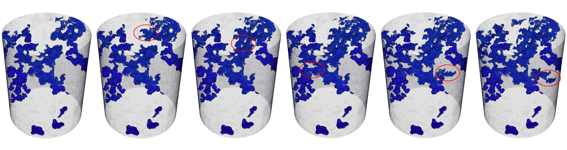
0:31:13.8: We do a lot of work with fluids as well in the systems, here's an example where we're looking at essentially oil going into a sandstone that's been permeated with a brine solution. This is quite important in the oil and gas arena. If you weren't aware of it, the majority of oil that's extracted from the ground today is pushed out by pushing something into the ground. So it's very important to understand the dynamics of different multiphase flow related to porosity and networks within rocks. So what we're seeing here, essentially a sample that's filled with brine and we're pushing oil into it, and you'll notice maybe during the animation that the filling was not a continuous event. It was discontinuous, you have networks that sudden... Or areas of the pores that suddenly quickly filled, these are called void jumps, and they are important to understand, specifically to understand the relationship between the liquids. Because the thing that you don't wanna do when you're applying this process is trap the oil.

0:32:20.1: Basically, you surround the oil with your brine solution and you can make it completely inaccessible. And there's literally billions of dollars involved in the differences in percentages of change. So it's really interesting. This is a nice sample to illustrate something called sliding window reconstruction. So in this sample, we did 12 seconds per rotation. So one might think, "Okay, well, we can see change in 12-second intervals." However, we have this full stream of projection data, so what we can do is we can actually slide our reconstruction window around and do some overlap of reconstructions to give us a bit more temporal resolution information here. So if we were stuck with 12 seconds, we'd have 0.8 here where we have a pore that's empty, and then we have point D where now it's completely full, and we just know that sometime in that timeframe, we went from empty to full. But if we can slide our window of reconstruction around a little bit, we can learn a little bit more. So here we've shifted it and overlapped by about four seconds.

0:33:27.7: So now we can see more clearly that, ah yes, the filling is actually happening a bit more in the second half. So now we can go back and look at the geometry of those pores and understand better the overall filling process related to the geometry of those pores because we have a bit more information in terms of the rate of fill. It's really also very, very useful to be able to visualize these changes when and where they happen. So this is just a snapshot of three different major pore-filling events, you see here circled on the graph here and visualized in 3D. And we have some nice tools to do this a bit more automatically in terms of labeling this in time and space. I'll talk a little bit more about that. But without those tools, it would potentially take several weeks to actually slog through the data to get to a point where you can visualize this in a meaningful manner. What's nice about that is, from the standpoint of doing it quickly, is that sometimes your experiment may not have gone the way you wanted to, but you may not know that until you've looked at the data.

0:34:41.5: So the sooner you can look at the data and understand from a temporal and spatial relationship when and where things are happening, the sooner you can maybe go back and redo it if you need to. In this particular case, it's interesting, we have a major filling event towards the early part of the results, towards the edge of the sample. This might have meant that our confining pressure was not quite good enough and we were actually getting flow around the side of the sample. So not necessarily desirable. It would be certainly much nicer to know we had that condition early on in our experiment than weeks down the road, so we can re-do it. Here's another example similar to the last one but it's done a bit more recently, and it's really, again, pushing more of the boundaries. This is seven and a half seconds per revolution here. The previous one was 12 seconds. So this is a centered glass, which is sort of a proxy to sandstone, and again it's the same sort of experiment where it's infiltrated complete with brine and then we're pushing oil through the sample. A voxel resolution about 12 and a half microns, so quite good in terms of being able to look at the overall network in this material here.

0:35:50.2: I'm gonna fast forward a little bit, because what's cool about this particular experiment is after we've done basically filling throughout this whole region, we've stopped the experiment and then we're zoomed into a smaller region of interest to do some higher resolution imaging. So that's what we're gonna be seeing here is now four and a half micron voxel resolution here at about a one-minute scan time, so really quite fast still at one minute, but much higher resolution. You can see the different grayscales in here. Everywhere it's dark is where the oil is, everywhere it's an intermediate is where brine still exists, and then the rest of it is all the matrix. And at this resolution, you're almost able to start seeing more discrete details about the interfaces between the liquids. In fact, in some regions, you can almost maybe even determine some contact angle information. So the ability to do a zoom like this on a sample and still have scans that are relatively quick, so you can still see the process of the change effectively, is quite nice.

0:36:58.1: Now, moving on a little bit, this is an interesting case, where we did an experiment, took a small piece of limestone, subjected it to a corrosive environment, it's supposed to be indicative of maybe some of the pollution we might see, like this hazy day in Paris, but limestone is a very, very common building block, especially for some of the older buildings, the beautiful cathedrals and such that we see throughout Europe. But over time, it does degrade, it develops this gypsum crust on the surface. That crust is fairly weak, so it can be chipped off and it can expose the underlying layer, continue to erode. Additionally, the surface is very, very rough, so it's a natural capturing mechanism for some of the particles in the air, it causes the outside of the building to look like crap and essentially make it look pretty bad. So this is a much longer experiment, it's a time lapse experiment, it's almost kind of continuous acquisition in the fact that there were 30-minute tomographies over the course of four days, and we did about 140 of them.

0:38:00.0: But what was still key to this is that we were using our 40 toolkits to really manage the data here. So you see a nice 3D rendering of the sample here, the outer growth, this gypsum crust, you can see it kind of accelerate towards the end of the sample. It's really nice to look at the outside surface. What's even better is to look at the inside surfaces. So here on the bottom, we have a difference map, basically the initial state divided by the ongoing state. So anywhere we see darker areas, that's a depletion of material from the substrate, and everywhere we see brighter material is growth of new material.

0:38:39.5: What's nice about looking in this way is that some of the changes in the actual data might be pretty subtle in terms of the grayscale change, and in fact, a lot of this is sub-resolution porosity happening. But because the material is becoming less dense, it's less attenuating, and we can actually detect that change in here.

0:39:00.7: Of course, we are a company that sells FIBSIMS and the Plasma FIB in particular is quite interesting for this case. What I expect would be an interesting experiment was to take something like this, do our time lapse series or a dynamic scan or this time lapse, I guess in this case, but then look at regions where we might have noted some significant changes in terms of rate and stuff like that and then use our CT data to help inform us of where to go with our Plasma FIB where we're able to actually access these areas effectively because of its capability to excavate large areas. So it's an interesting correlative project. We would, of course, like to look at that in grayscale and it's nice to look at, but we also wanna understand in a slice view, but we also wanna understand volumetrically how things are changing and since this is a time domain we're talking about, we really wanna understand when things are changing.

0:39:58.0: From the overall histogram, we can clearly see changes happening related to the different minerals and materials within the sample, but this is kind of a generalized view of things. So what we end up doing is this process called flip point detection where we actually track a voxel or a group of voxels from volume to volume and then basically timestamp when those voxels or that voxel changes grayscale and then this now allows us to understand the temporal nature of the samples. So in the earlier example with the oil and brine, I showed this rendering showing these different filling events at different times and this was easily visualized in that 3D image. This sort of technique, the flip point detection, is how we can get to that result relatively quickly.

0:40:53.8: So for here we did the same thing and now what we're looking at here, this grayscale now represents basically when things happened, not exactly... Not the change in material specifically of erosion or depletion or growth material, but it's when it happened. So now in the colorized version, it's quite easy to see that changes that are in blue happened earlier in the process, changes in red happened later. The size of the color band also has some indication of the rate of change at that time too, so it gives us a nice snapshot of when and where things are happening as this thing evolved. And then of course, it is 3D data sets, so we wanna be able to visualize this in 3D, kind of accumulating all of the data in one snapshot and giving us a nice idea of how this thing has evolved over time.

0:41:45.9: Alright, switching gears a little bit here. The guys in the lab, in our apps lab in Ghent, decided to literally watch grass grow in the system, so they put these little cress seeds in there and they watched as they sprouted. So they did this experiment where they watched how they sprouted for several days, so they watched them grow and then they did a more dynamic experiment looking at just the initial early stages when the sprout is first coming out of the seed. So that first video here... Oops, gotta replay, there we go, is of the full kind of growth over several days. Just a five-minute scan basically every hour. We didn't wanna do much longer. You don't wanna subject these things to too much X-ray because they are living, so that can have an adverse effect. It's a lot of interesting detail here. You might have noted that towards the end of this growth, there are a bunch of little hairs growing towards the bottom of these sprouts. At first I thought that was actually part of the sprout, but then I was later better educated that it actually is some mold growing in there. So it's cool that we can see these different things happening in the system here.

0:42:57.3: On the dynamic side, as I mentioned, we... Whoops. Let's play that again. We just really focused on this first portion of growth where the sprouts are coming out of the seeds initially. So just to give an insight about what's happening really in that point. It's just a four-hour experiment. This one, again, continuous and not interrupted, not at a certain time interval, but a continuous acquisition.

0:43:22.6: Moving into something a little more tasty. We've done some experiments and some imaging of some food products, most notably some interesting baking experiments. First one here is of a little muffin, so on the left here, you see a virtual cross-section of the sample. Again, fast scans, order of 11 seconds. When we're dealing with this type of material, it's typically gonna be a little coarser resolution because it's lower attenuating. We'll need a little bit higher signal to noise in order to do these fast scans, which has a trade-off a lot of times of being a little bit coarser resolution. However, for this particular sample, the resolution is quite sufficient in order to see some of these bubble formations do some rendering of these so you can see the actual change in the bubbles during the process. You can see the little foil that it's sitting in.

0:44:15.5: We learned after the fact in a little more investigation into muffins that muffins have a very particular type of pore structure that are special to muffins, different than you might have with other baked goods. So you learn new stuff about different things all the time in the CT world. Well, here's another baking experiment, this time of a croissant that started in a frozen state, put into an oven, ramp the temperature up, and then we see first the thawing of the croissant and then the nice baking out where it gets a lot puffier. I'm always impressed about the amount of interest in microstructure into food. Years ago, I once imaged a Cheerio, breakfast cereal, so one of the Cheerios from breakfast cereal, the little Os. And I asked the gentleman why he was interested in looking at the inside of this Cheerio and he said, "Well, water is cheap and air is free, so if we can put more of those into the product, we can make it for cheaper and we can sell it as a healthier option." So some interesting stuff going on.

0:45:19.9: The other part about it is also the mouth feel. So when you're making, in general, healthier products, you want it to taste like the original or feel like the original. So let's say you're doing a potato chip. We imaged a lot of potato chips back in the day. You really wanna understand the distribution of the different components in that microstructure specifically so that it feels the same in the mouth 'cause that's a big important part of our whole eating experience. So pretty interesting stuff.

0:45:50.4: This next example, certainly, I think is one of my favorites lately, is this one in the DynaTOM where we put a cone of gelato or ice cream in there, and we imaged it as it was melting. So you'll see here on the left, nice 3D rendering of the sample as it's melting, the match up of the melting process and the data acquisition is quite nice in this case, it's very smooth and you can see a lot of detail about how this is proceeding, in this case we're doing full scans in about 12 and a half seconds, but we were reconstructing only half of that, so 180 degrees, so we were essentially able to double the temporal resolution in that case. Here are some cross sections from that same sample, interestingly, the chocolate chunks inside are much denser than the surrounding ice cream material, and then on the outer surfaces, you can really see where the melt region is happening with this pore porosity happening in that melt region, so really cool stuff.

0:46:47.7: Alright, my last example, if you guys have seen any of these dynamic CT presentations by us in the last couple of years, you've probably seen this example, but it's still one of my favorites, it's looking at beer foam, so beer is near and dear to the hearts of the Belgians, so it's natural that we would try to do some investigation involving beer. In this case, we put a glass of beer into the DynaTOM and looked at how the foam degraded over time. In this case, it's pretty coarse resolution, 150 micron, again, it's a very low density material, so you'll again, need to do a bit higher signal to noise to get decent images. I will tell you that this is a plastic glass, not a regular glass, because a regular glass would be even more difficult to penetrate through for this live material, but it's still really, really nice data. Here's a quick video of our applications, Engineer Frederick placing the sample in the system. You can see that there is quite a large head on the sample, which certainly is intentional for this particular experiment, but I think it hurt these guys to actually pour that foam so big, it's such a... Beer is such an important part of the culture there, they told me that if a bartender were to pour this beer like this, they would risk losing their job, it's that dire, they really are very much focused on having good pours in every single beer, so it's a funny little factoid.

0:48:15.2: We did some interesting analysis of the foam with some software where we imaged over three million pours throughout the data sets, and we didn't just do one beer, we actually did two beers, so we have a comparison of the two in both quantitatively and qualitatively, the difference is abundantly clear, vastly different size of pours in the foam, the dissipation rate is much, much different between the two, when I first joined TESCAN and started getting in these dynamic stuff, this was the big reason why I joined, is because this dynamic stuff is very exciting and it's new, I spent a lot of years working in kind of the high resolution area, and they showed me this example and I was blown away by the ability to capture this sort of data, and then I said to myself, "Well, what's important about looking at beer foam?" And I thought about it more, I realized taste and smell are closely linked, so if you have a foam, it sticks around a little bit longer and you capture some of the aromatics of the beer, especially in our day of craft beer, with a lot of interesting flavor profiles, your beer drinking experience will be more consistent through the whole beer, so from one standpoint it's definitely an important part of the overall experience in drinking your beer.

0:49:36.2: Alright, well, I thank you guys for taking the time to listen about dynamic CT, this and other webinars will be available as recordings later on, and I re-recorded my intro one just yesterday, so that'll be available at some point. In general, I wanna just say that our goal at TESCAN from the micro-CT side is really to enable this idea of dynamic CT imaging, make it more commonplace and routine technique in the lab. Our products are really engineered with this in mind, they're very capable of doing nice imaging for static single samples, for large samples, a multi-scale, but really by coupling software, hardware and experience together, we're hoping we can enable a new era of dynamic CT imaging. With that, I'll just stop on this slide where it shows the rest of the different learning labs that are available, I don't have the dates on this slide, but basically, we're here on Tuesday and we're gonna be running them more or less every week for the next couple more weeks, and wherever you registered for this one, you should be able to register for these other ones that'll give you more information about some of our FIBSIMS, SEMs, and that sort of thing, if you have any specific questions that you don't wanna ask in this regime, in this arena, and you wanna contact me directly, my email is down here at the bottom, luke.hunter@TESCAN.com, and with that, hopefully Hope is back online here and we can go ahead and see if there were any questions.

0:51:12.1: Thank you Luke. We have a few questions. The first is, "What is the reconstruction software being used?" And that came in early and in your presentation probably when you were talking about LEGOs.

0:51:25.4: Okay, yeah, so we actually use our own reconstruction engine in-house, so from the standpoint of doing the reconstruction from 2D to 3D for visualizing the data, where you will use our own internal 3D viewer, Pantera or we'll use a third party software we... One of the software packages we end up using a lot is called Dragonfly from the company ORS, but for the visualization analysis that's typically with a third party, the reconstruction though is with our own software.

0:52:03.3: Thank you. The next question is, for small biological specimens such as insects, a lot of micro-CT work has been done using the Bruker SKYSCAN system. So how does the test scan model compare or differ? 

0:52:20.3: So Bruker has a wide range of systems. A large number of their systems are desktop, and for small insect imaging, they have options for certainly higher resolution. We're not really focused as much on the higher resolution at this point, we're really focused on this dynamic CT capability and flexibility for larger samples, so our systems have spatial resolution about three micron, Bruker and other vendors will have systems that go to a higher resolution. They're significantly different, certainly, our systems will typically be much, much higher power in terms of the X-ray source and much faster detectors as compared to some of these other systems, so we can certainly do a nice job of imaging insects down to a certain level of resolution, but there are some other options for doing higher resolution out there right now.

0:53:15.3: Okay, the next one, what is the smallest feature you can resolve both in dynamic and static experiments? 

0:53:23.3: So our spatial resolution for our system is specified at three micron and that's, again, spatial resolution. So you always need to make sure the distinction between voxel resolution and spatial resolution is pretty clear, some folks quote "voxel resolution" as their main resolution specification, but you just have to be aware that its overall system resolution is a function of multiple factors, and voxel size is just a function of geometry. So you have to be aware of those differences. In a static scan, yeah, so we can scan down on the order of one to one and a half kind of micron voxel size, maybe smaller in some cases, which would be about a three micron spatial resolution. In the dynamic world it's always gonna be a trade-off about how fast you go. So in this presentation, I had an example where we did about a four and a half micron voxel size, which should relate to about a 10 micron kinda spatial resolution somewhere in there in terms of seeing features, there's also a difference between detectability and true spatial resolution, if you have very small particles that are high density, you'll be able to detect those even though they might be smaller than the voxel, so it gets a bit complicated. But in general, the dynamic side is gonna be a little bit coarser, and it's gonna be dependent on the type of sample you're using and how fast you wanna go.

0:54:53.4: Okay, what is the best resolution of the system? 

0:54:57.2: So I think I just covered that in the last question, basically. Yeah, three micron, spatial resolution at this point. We certainly have... We're looking at other possibilities down the road of something providing a bit higher resolution, but right now our offerings are in that range about three microns spatial resolution.

0:55:17.1: Okay. For your detector, do you only use flat panel detector? 

0:55:22.4: In the current systems? Yes. Yeah. We're really focusing on very fast scans, in fact, the detector we use in the UniTOM XL and CoreTom is a very fast detector, it can go up to 100 frames per second when it's in a windowed and bend mode, so it's certainly very, very important for doing these dynamic acquisitions. You need to be able to have a detector that has a very fast read out speed in order to collect data fast enough to do scans in the order of six seconds or 10 seconds or something like that. When we're collecting still hundreds, if not 1000 or so projections in one of these datasets.